Backpropagation Gentle Introduction

Backpropagation is a way to compute the length of the cost-optimization step.

Take Info → Do some magic → Give output → Calculate the mistakes (errors) → Optimize the magic → Repeat

1. We took the inputs.
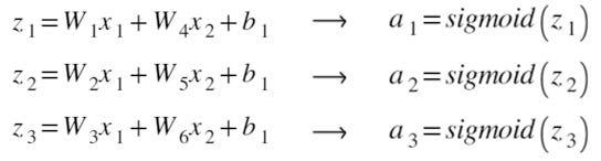
2. We performed Forward Propagation.
3. We computed the Cost Function.
4. We performed Back Propagation.
5. We performed Gradient Descent to optimize the parameters (weights and biases).
6. Repeat from step 2 until the desired results are achieved.

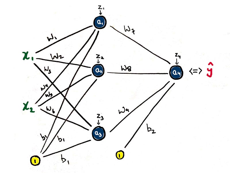2-L Basic Neural Network

Layer 1

Layer 2

Now,
    y → original labels
    y_hat → predicted labels

and here, m = 1

Therefore, total error,

Now, we’re left with just one tini-tiny job (haha), i.e. to find the ‘change’.

Enters Backpropagation.

If you’re anything like me, I’m sure you too have a hard time understanding what exactly ‘derivation’ means. Whenever I asked my teachers, they would just say that it’s the slope of the tangent …or …or the rate of change …or breaking down value into smaller values. To be honest, I never understood it, until I came across backpropagation.

Let me put it this way, say you’ve got a car. A car’s speed depends on what? On a higher level, it’s engine (duh!), wheels and maybe spoilers (tell me if I’m wrong, not a car expert you know!). So now, we’ve three components that affect the speed of the car.

Now, one question, how will the speed of the car be affected if I change the engine? Ok, let me put this another way, we have to find the change in speed w.r.t the engine, right?

Now, let’s add maths to the mix.

Let ‘v’ be the speed of the car,

e → engine, w → wheels, s → spoilers

So,

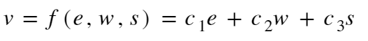c1, c2 and c3: constants

NOTE: Here, we’re using a special type of derivation called Partial Derivation, which is basically used when a function depends on multi-variables (here, e, w, and s).

Therefore,

I hope you guys got a little intuition of what exactly is meant by derivation. Ok then! Let’s move forward…

Now the big question arises, on what variable/parameter does the error even depends? Let’s backpropagate (pun intended ;)

How did we reach our error? Cost Function? Right.

What does Cost Function depend on? Original and Predicted labels? Right. Can we change the original labels? Duh! NO! What’s left? Yes, Predicted labels.

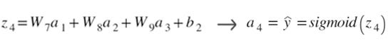
Now, we’ve rolled back to our forward propagation step. How did we reach predicted labels again?

Here we see that the Forward Propagation basically depends on the inputs and the weights we initialized. Are you getting what I’m trying to point at? We cannot change the input (how convenient would that be if we could? Imagine!). So, we’re only left to tinker with the weights and biases. That means, they can be customized as per our convenience, so…let’s!

Now to see how W_7 is affecting our cost function (remember the intuition?), let’s take the help of Miss. Maths,

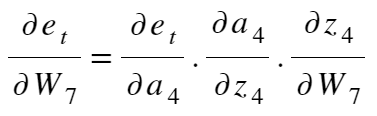The derivative can be expanded like this, right?

now, let’s solve it term by term,

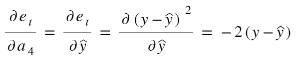note, a_4 = y_hat

Derivative of Sigmoid

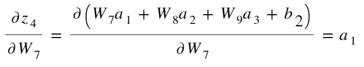expanding z_4 as in Forward Propagation

For simplicity, let’s just say we’ve got dW_7 (rather than saying it de_t/dW_7).
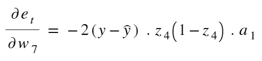
Now, we just repeat this process w.r.t every weight (W1-W9) and every bias (b1 and b2) to find respective derivatives.

Now what? See, we’ve got the change in the parameters that we wanted ever since the beginning of the article. Now we just need to update the respective parameter.

Not so fast kid!

See, if we only talk about Backpropagation functionality, then we’re done. The sole purpose of backpropagation is to just calculate the change to be made. Updating parameters is whole another step.

And that step is, ‘Gradient Descent’.

Gradient Descent and Backpropagation (Intuition):

In a nutshell, Gradient Descent is the most basic optimization algorithm which takes some calculated steps towards the minima of the Cost Function, until it converges. Thus, minimizing error and maximizing accuracy!

What Gradient Descent basically does is that it updates the value of a weight/bias.

Gradient Descent takes a parameter called ‘Learning Rate (alpha)’. Now, this is interesting. Learning Rate decides how big steps the function will take towards the minima (or sometimes even away from the minima.)

Now I know what you’re thinking. First, we did Backprop to find the change, and now we’re saying that the learning rate decides the change, what is this fiasco?

Stick with me for just one more minute.

So basically, the derivative we got from Backprop decides in what direction we need to move (obviously towards the minima, but the minima could be either at left or right of the current position, right?) and the learning rate determines how fast or how big steps we are taking towards that direction.

Learning Rate Fiasco: There’s a catch with Learning Rate (alpha) which I think I should tell you right away quickly. See, if we set alpha to be very small, our function will take a very long time to converge to the minima and on the other hand, if we set it high, our function might never even converge! The following gif will make things clearer.

Small Learning Rate

Large Learning Rate

So, generally, the value is taken among the following :
alpha ≥ 0.001, 0.003, 0.01, 0.03, 0.1 ≥ alpha
And of course, you’re all allowed to take any value and check what works best for you.

Now what, we’ve calculated everything we need for Backpropagation. We just need to update the parameters using the above Gradient Descent Equation.

Now if we go back to the workflow, we’ve Optimized our function, and now to until the desired results are reached, we have to iterate (repeat) the workflow again and again and again and again and again and again and again……

More Machine Learning Deep Learning Resources to refer:

 

• Machine Learning Deep Learning Best Courses
• Machine Learning Deep Learning - Siraj Rawal

 

More Machine Learning Deep Learning Books to refer (Very Popular):