aiartificialintelligencebigdatacomputersciencedatadatascienceDeep LearningdeeplearningFutureiotmachinelearningneuralnetworkspythontechnology
Neural Network in Machine Learning in a Nutshell (from Scratch)

Oh, you’re still here? Wanna know more? Ok then, hop in.
Just like a baby tries to stand or walk or use hands effectively or laugh or anything, it does not do it perfectly in the first attempt. It does something, it fails, it learns from its mistakes, takes our feedback and then does it again. And on the millionth try (damn that kid!), it succeeds!
Neural Network is just the same. It’s a model that tries to do something (mainly, predictions), fails at first, considers its errors and sometimes our feedback too (tuning the learning rate, we’ll come back to it later) and then tries again. And not in a millionth try (hopefully!), but after some tries, or let’s be a little technical over here, after some iterations, it finally gets better at its job.
I’m assuming you’re a layman so I’ll be explaining from basics in simple terms. What? You already know that? Well, you can totally skip ahead for the main treat.
The term “Neural Network” did not come from anything outside in the world, but from within us only. Our brain, the complexity king, contains billions of ‘Neurons’ which are nothing but basically nerve cells that are the basic building block of our Nervous system. But unlike other cells, Neurons are specialized to transmit information throughout our body. Well, let’s not go deep into the bio, it’s not a bio class after all (I’ve always hated bio!). So, Neural Nets are just an attempt to replicate the Neurons in our body. The stripped-down process of a Neural Network is:
Workflow (Neural Network Algorithm):
Take Info → Do some magic → Give output → Calculate the mistakes (errors) → Optimize the magic → Repeat
Now that you know the basic structure, let’s dive a little deeper!
Basic Building Block: Neuron
A Neuron (sometimes also referred to as a Node) is the smallest element of a Neural Network. Its basic functioning is to take some input, do some math-a-magic and then spit out some output. There we go, that’s it!
As you can observe, there are a few things that are happening here:
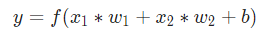
1. Each input is being multiplied by a Weight
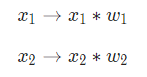
2. The weighted inputs are being added together with an extra term, bias.

3. Finally, the sum is passed through an Activation Function.
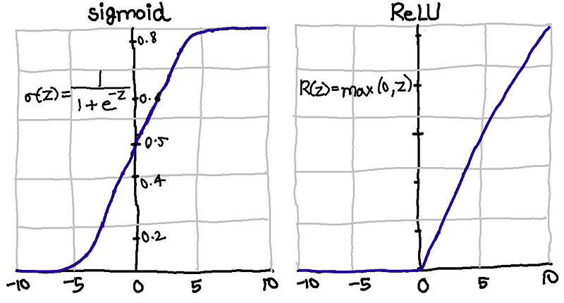
Activation Functions:
An activation function is nothing but just a way to convert the inputs into a nice and scaled output which works better while predicting in a Neural Network training.
 |
| *not to scale |

Simple Neural Network example:
Building a Neuron from Scratch in Python :
Great! We’ve implemented our first Neuron! Welcome to Machine Learning! And now that you had a little taste of it, let’s move forward to what exactly Neural Networks are.
Neural Network Definition
A Neural Network is nothing but just a bunch of Neurons packed together in some structure. Seriously!
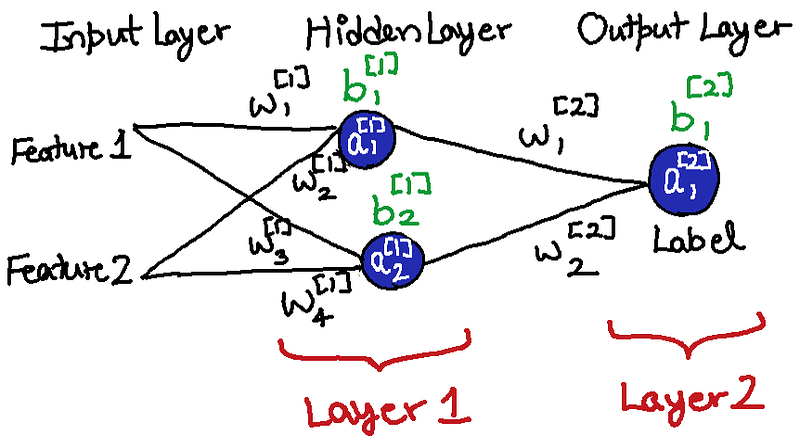
As we can see, a NN is mainly divided into 3 parts:
- Input Layer
- Hidden Layer
- Output Layer
Input Layer is the Input data we feed to a network that we want to do our predictions on.
Hidden Layer takes input from the Input Layer and then performs the math-a-magic and then spits out some numbers.
Output Layer takes the output of the Hidden Layer as input, does the math-a-magic again and then spits out the result. Cool..! Right?
And this my friend is nothing else but the complete Feed-forward Algorithm !!!
Note: The most basic NN is a 2-Layer NN with only 1 Hidden Layer. Though there can be multiple hidden layers, but only 1 Input and 1 Output Layer.
Therefore, the total number of layers, L = n Hidden Layers + 1 Output Layer
Though, the basic idea remains the same. Feeding the input(s), feed-forwarding through the neurons in each layer towards the output and getting out the predictions.
Representing the Dataset
We, for the sake of simplicity, will use a very basic Dataset.
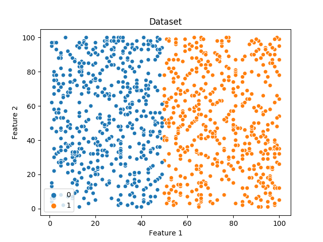
Here, there are two Features and one Label. Can you observe how the labels have been marked?
Now, we have our Dataset and we have our NN structure too, what’s left? Yup….TRAININGGGG!!!!!
Feed-forwarding in Python
Awesome! Now that we’ve got our first predictions, let’s check our performance and move closer to optimizations (getting more accurate).
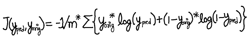
Cost Function:
Ok then. Things are gonna be a little trickier from here on. So, tighten your seatbelt. Vroom..!
Now that we’ve reached our first solution (hey man, the first solution? What do you mean by that? Don’t worry. I’ll explain everything). So where were we, yes, once we reach our first solution (hey man, the first solution? What do you mean by that? I said don’t worry. I’ll explain everything. Ok?). Ya, so, first solution…(umm…dude..? Arrgh! Shut the…).
We need to compute Loss! We need to come up with some way, some formula, some function to check how well we did. No, we can’t do that just by looking manually and comparing. Yes, we can do it in very small datasets with up to 5–10 examples (like our dataset), maybe even up to 15. But what will you do when the number of examples crosses 100? What about 1000? Tens of 1000s? A million?
Yes, the dataset CAN BE that big! Did you forget already? The more the Data the better the Machine Learning Model!
Enters Mr. Cost Function.
If you haven’t guessed it by now, Cost Function is a function that helps to compute the error in the predicted values. It is also represented by ‘J’ in mathematical representations.

Well, this is it. Simple isn’t it? Let’s just break it down to understand,
- m: Number of examples our dataset has.
- y_pred: The predicted labels (yhat, according to our code.).
- y_orig : The original labels, y.
- Σ: It’s a mathematical character that means ‘to take sum of’. (You’ll get it later. Chill.)
(y_orig - y_pred)^2 : It is known as the Squared Error.
C’mon, c’mon. Use your brains now. If that term is called Squared Error, what happens if we divide it with the number of examples? Huh? C’mon c’mon. Try.
Well, there’s no way for me to know what you answered, but if you said it’ll make the values smaller to work on, haha…
NOT AT ALL!
It converts the Squared Error into Mean Squared Error. Ok ok, I’ll explain. See, our loss function J here is simply taking the average over all the squared errors. Thus, ‘Mean’ Squared Error.
The better our predictions are, the less our loss will be. Or we can also say it like this,
The less the loss, the better the predictions.
Therefore, we only focus on one and only one thing while training a Neural Network. We try to minimize loss, cause that automatically gives us better predictions with higher accuracy.
Cost Function from Scratch:
Now that we’ve got a way to calculate the error, the only steps left now are to work out some way to minimize the error.
Neural Network Backpropagation:
Now, we’ve got a clear goal, don’t we? Minimize the Cost Function. But how do we do that?
To answer that, let’s take backward steps and see how we reached that stupid Cost Function in the first place anyways:
- We took the inputs.
- We generated some Weights and biases.
- We multiplied the Weights and inputs and then added the bias, followed by feeding the output to some activation function. Basically, Feed-forwarding.
- We calculated the output of the final layer (output layer).
- We then computed the Cost.
So this was the progress we made so far right? Cool then. What next? And why did we went through the steps?
The answer is simple. What I want you to recognize in the above step the things/process which were in our hands. The things we could’ve have altered with.
We cannot change the input, obviously! You can’t change the question if you’re not getting the answer right. As simple as that! (Or can you?)
Secondly, we cannot tinker with the activation function. C’mon, it predefined.
So what can we do..? Tell me, what we want to do in the first place? Ya, minimize the Cost Function. Now tell me, what is influencing the Cost Function? There we go, the predicted output (’cause the other thing is the original label and that is fixed.) One last thing, how did we reach that particular predicted output? Yes? Yes? Yes, through Feed forwarding. And now the ultimate last question, what all things did we use in our Feedforward algorithm..?
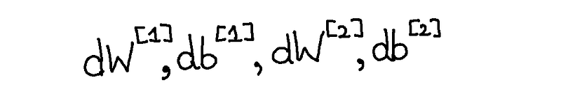
Yup, you got it right! We can very well play with the Weights and biases that we generated ourselves. That means, they can be customized as per our convenience, so…let’s!
So, after having a dinner date with calculus, she gave us a present before leaving. She gave us a couple of parameters;
dW and db (for each respective layer)
So now, we’ve with us :
Now that we’ve got the required changes we need to make to the Weights and biases, let’s change ‘em.
Ho Ho Ho, not so soon my friend, there is one last tini-tiny step remaining.
Gradient Descent:
If you’ve never heard of this term, I bet this must be scaring you. Have no fear thy friend, this might be the easiest thing to implement so far. Betcha!
I’ve already explained Gradient Descent in details, but to give you just a quick overview,
It is a process of finding the minimum value location of the Cost Function when plotted against Weights. And, how big steps we’re taking towards the minimum is determined by the parameter ‘Learning Rate’.
 |
| Gradient Descent |
So if we iterate this over every Weight and bias correctly, we’ll see the Cost Function Graph decreasing over every iteration (hopefully!).
Baking the Pie:
Now let’s recall what was the Workflow of the Neural Network:
Take Info → Do some magic → Give output → Calculate the mistakes (errors) → Optimize the magic → Repeat
But now we’re not dumb as before, now we can use the correct technical jargon. So, defining the workflow again:
Taking Input → Generating random Weights and biases → Predicting the labels using Feed Forward → Compute the Cost Function to keep track of Prediction Error → Calculate the small changes to be made using Back Propagation → Updating the Weights and biases using Gradient Descent → Iterating over the process to reach the desired accuracy
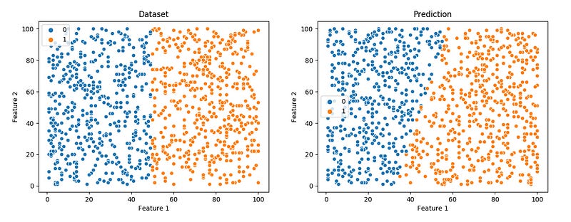 |
| Original Labels v/s Predicted Labels |
 |
| This kind of Cost Function slope represents that everthing went well! |
Now, why don’t you visit my playground and give this a go yourself? Try to come up with better accuracy by tinkering with the parameters, and tell me in the comments if you get some good results!
And if you want the complete code, head over to my GitHub Repo (it's slightly changed though, but'll it won't be a problem 'cause you're a pro) and have fun!
Peace out.
And if you want the complete code, head over to my GitHub Repo (it's slightly changed though, but'll it won't be a problem 'cause you're a pro) and have fun!
Peace out.
I want to thank my good friend, Naveen Goswami, for helping me out with the diagrams with his amazing drawing skills. Thanks man, for staying up late with me to complete the job (without even any pay! haha). Thanks again, and I might need your help again so, buckle up!
More Machine Learning Deep Learning Resources to refer:
More Machine Learning Deep Learning Books (Very Popular):

0 comments